Example 00: Isotropic Checkerboard

This example reproduces the SurfATT/examples/00_checkerboard_iso workflow. It builds a synthetic isotropic checkerboard model, calculates Rayleigh-wave phase travel times, and inverts the synthetic data to test how well the three-dimensional velocity pattern can be recovered.

What is included

Parameter setup

The default configuration uses:

• isotropic inversion (model_para_type: 0)
• Rayleigh-wave phase-velocity data
• model depth range of 0-15 km
• longitude, latitude, and depth intervals of 0.02° / 0.02° / 0.5 km
• linear initial model with vel_range: [1.8, 4.2]
• up to 40 LBFGS iterations

Topography is disabled in this example.

Run the example

The example has two dependent stages. First, SURFATT_cb_fwd creates the target checkerboard and calculates synthetic observations. Then, SURFATT_tomo starts from the unperturbed model and attempts to recover the checkerboard from those travel times.

From the example directory, the supplied script runs the complete workflow:

bash run_this_example.sh

The following sections unpack the script step by step using the current executable names.

1. Prepare the forward input

Create the output directory and copy the source–receiver geometry to the filename configured for Rayleigh-wave phase velocity:

mkdir -p OUTPUT_FILES
cp src_rec_file_ph.csv OUTPUT_FILES/src_rec_file_forward_RL_PH.csv

The default data selection is:

wave_type: [True, False] # Rayleigh only
vel_type:  [True, False] # phase only

At this stage, the copied CSV file supplies the source–receiver geometry, periods, and data weights. Its travel-time and velocity columns are replaced by synthetic values during the forward calculation.

2. Generate the target model and synthetic data

mpirun -np 8 ../../bin/SURFATT_cb_fwd \
  -i input_params.yml \
  -n 2/3/2 \
  -m 0.2 \
  -p 0.08

The forward command creates a 2 × 3 × 2 checkerboard: two anomalies along longitude, three along latitude, and two in depth. Adjacent anomalies are separated by a 0.2° horizontal margin and alternate between positive and negative 8% $V_s$ perturbations. SurfATT then calculates Rayleigh-wave phase travel times through this known target model and writes them to src_rec_file_forward_RL_PH.csv.

The horizontal target slices show the alternating checkerboard polarity at 3.5 and 11.0 km depth. The sign reverses between the shallow and deep layers, as expected from the two-layer checkerboard definition.

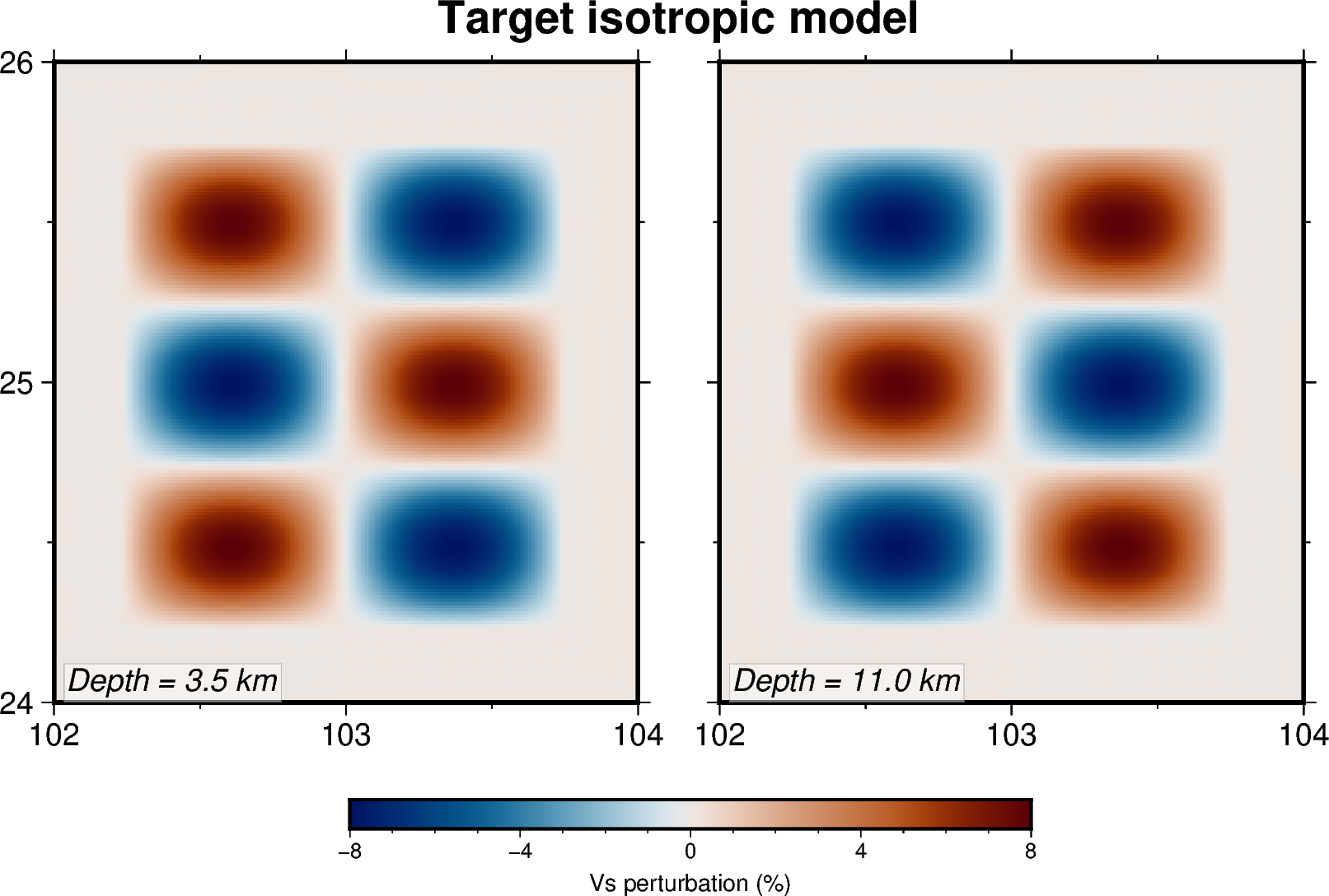
Target $V_s$ perturbations at 3.5 and 11.0 km depth.

The two target cross-sections cut through the model at latitude $24.99^\circ$ and longitude $102.59^\circ$. They expose the alternating anomalies in both horizontal directions and show the separation between the shallow and deep checkerboard layers.

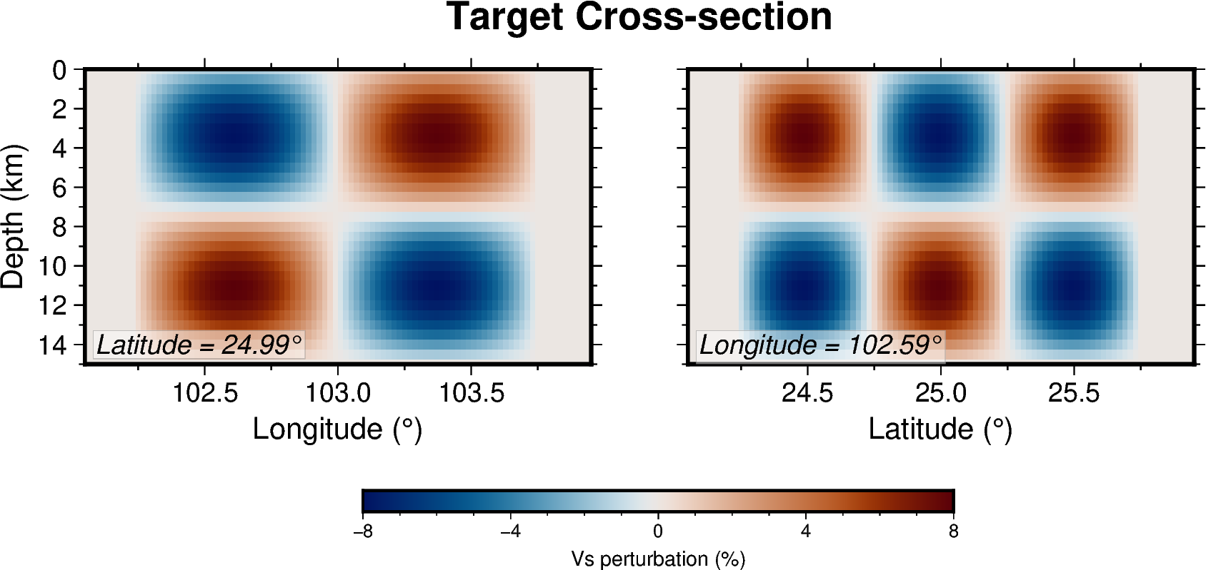
Target $V_s$ sections at latitude $24.99^\circ$ and longitude $102.59^\circ$.

The main products of the forward stage are initial_model.h5, target_model.h5, and the synthetic observation table src_rec_file_forward_RL_PH.csv.

3. Invert the synthetic observations

After the forward calculation finishes successfully, run:

mpirun -np 8 ../../bin/SURFATT_tomo -i input_params.yml

The inversion rebuilds the unperturbed starting model and predicts travel times for the current model. At each iteration it calculates travel-time residuals, forms the adjoint $V_s$ sensitivity kernel, applies the configured PDE smoothing, and uses LBFGS with line search to update the model.

The run stops after niter: 40, when the recent mean-misfit reduction falls below min_derr, or when the line search can no longer find an acceptable update.

Expected outputs

After the run finishes, inspect the OUTPUT_FILES directory for:

• initial_model.h5: unperturbed starting model
• target_model.h5: checkerboard model used to generate the synthetic data
• final_model.h5: recovered isotropic S-wave velocity model
• model_iter.h5: intermediate models written during inversion
• objective_function.txt: misfit history for each iteration
• src_rec_file_forward_RL_PH.csv: forward-calculated Rayleigh-wave phase data

Visualization

Open plot_model.ipynb to reproduce these figures or inspect other depths and sections. The notebook compares initial_model.h5, target_model.h5, and final_model.h5 and calculates the recovered perturbation relative to the initial model.

The recovered horizontal slices preserve the anomaly locations and alternating polarity of the target checkerboard. The shallow 3.5 km layer closely recovers the imposed amplitudes, while the 11.0 km layer is weaker and smoother because deeper structure has lower travel-time sensitivity and is more strongly affected by regularization.

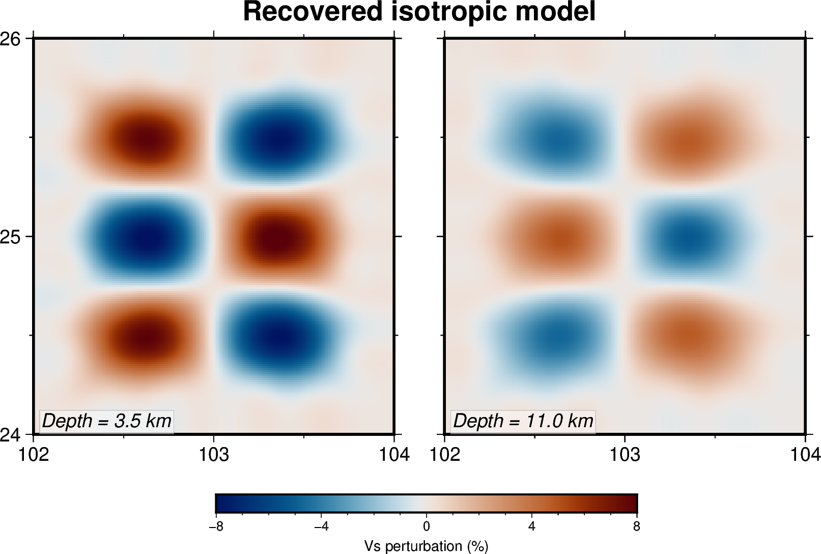
Recovered $V_s$ perturbations at 3.5 and 11.0 km depth.

The recovered cross-sections retain both checkerboard layers and the correct anomaly polarity. Recovery is sharpest in the shallow layer; the deep anomalies have reduced amplitude and broader boundaries, particularly near the edges of the model where ray coverage is less uniform.

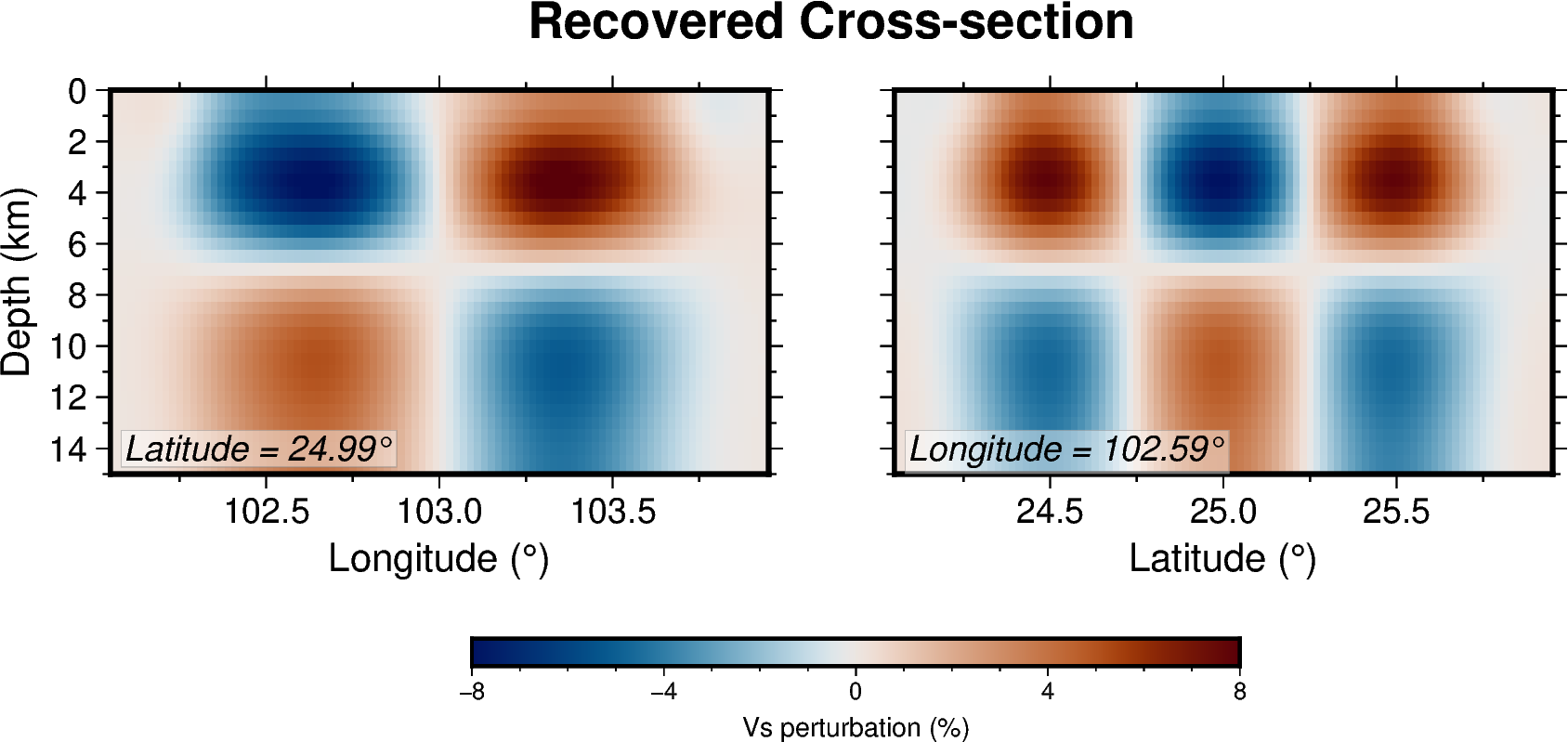
Recovered $V_s$ sections at latitude $24.99^\circ$ and longitude $102.59^\circ$.

For a quantitative assessment, compare target_model.h5 and final_model.h5 using the same color scale. Check the recovered anomaly polarity, location, amplitude, vertical separation, and any smearing between neighboring blocks.