Example 01: Azimuthal Anisotropy Checkerboard
This example reproduces SurfATTPP/examples/01_checkerboard_azimuthal_ani. It tests whether the inversion can recover an isotropic checkerboard together with an independent azimuthal-anisotropy pattern.
Model parameterization
SurfATT represents azimuthal anisotropy using an isotropic S-wave velocity and two orthogonal anisotropic coefficients:
| Parameter | Unit | Definition and physical meaning |
|---|---|---|
| km/s | Isotropic S-wave velocity that controls the azimuthally averaged structure | |
| dimensionless | Cosine component of the azimuthal variation | |
| dimensionless | Sine component of the azimuthal variation | |
| dimensionless | Azimuthal-anisotropy magnitude | |
| degrees | Fast-axis direction, defined modulo |
The magnitude and fast-axis direction are derived from the two inversion coefficients:
Conversely,
The factor of two makes the parameterization periodic: and describe the same fast-axis orientation. When , the model is azimuthally isotropic and the fast-axis direction is undefined.
Internally, SurfATT directly updates , , and . The HDF5 model files also contain the derived g0 and theta fields, so users can visualize anisotropy as oriented bars whose direction represents and whose length represents .
What is included
| File | Description |
|---|---|
input_params.yml | Azimuthally anisotropic inversion settings |
src_rec_file_rl_ph.csv | Rayleigh-wave phase-velocity source–receiver table |
run_this_example.sh | Script for the forward and inversion stages |
plt_model.ipynb | Notebook for plotting and azimuthal anisotropy |
Parameter setup
The default configuration uses:
- azimuthally anisotropic inversion (
model_para_type: 1) - Rayleigh-wave phase-velocity data
- model depth range of
0-12 km - longitude, latitude, and depth intervals of
0.02° / 0.02° / 0.5 km - separate smoothing scales for and
- up to
80LBFGS iterations
Setting model_para_type: 1 activates the –– inversion. The current azimuthal-anisotropy implementation uses Rayleigh-wave phase velocity; Love-wave and group-velocity data must remain disabled.
Run the example
The example has two dependent stages. First, SURFATT_cb_fwd creates the target isotropic and anisotropic checkerboards and calculates synthetic observations. Then, SURFATT_tomo starts from an isotropic model and attempts to recover both structures.
For a complete automatic run, execute the supplied script from the example directory:
bash run_this_example.shThe following sections unpack the script step by step.
1. Prepare the forward input
Create the output directory and copy the source–receiver geometry to the filename configured in input_params.yml:
mkdir -p OUTPUT_FILES
cp src_rec_file_rl_ph.csv OUTPUT_FILES/src_rec_file_forward_RL_PH.csv
The default data selection is:
wave_type: [True, False]  # Rayleigh only
vel_type:  [True, False]  # phase only
At this stage, src_rec_file_forward_RL_PH.csv provides the source–receiver geometry, periods, and weights. Its travel-time and velocity columns will be replaced by synthetic values during the forward calculation.
2. Generate the target model and synthetic data
Run the azimuthal-anisotropy checkerboard forward calculation:
mpirun -np 8 ../../bin/SURFATT_cb_fwd \
  -i input_params.yml \
  -n 3/3/2 \
  -a 2/2/2/135 \
  -p 0.08/0.08 \
  -m 0.2 \
  -s 4
The command-line options define two independent checkerboards:
| Option | Meaning |
|---|---|
-i input_params.yml | Read the data path, grid, initial model, and output settings |
-n 3/3/2 | Create a 3 × 3 × 2 isotropic checkerboard |
-a 2/2/2/135 | Create a 2 × 2 × 2 anisotropy checkerboard with a reference fast-axis angle of |
-p 0.08/0.08 | Use an 8% perturbation and an anisotropy magnitude of 0.08 |
-m 0.2 | Leave a 0.2° horizontal margin between adjacent anomalies |
-s 4 | Set the upper anomaly size to 4 km |
The forward stage proceeds as follows:
- SurfATT builds the 1-D starting model and extrudes it over the 3-D grid. The initial anisotropic coefficients are .
- Alternating perturbations are added to using a
3 × 3 × 2pattern. - A separate
2 × 2 × 2pattern is created for azimuthal anisotropy. Positive blocks use a fast axis; negative blocks rotate the axis by , giving the orthogonal orientation. - The anisotropy magnitude and direction are converted to and .
- Rayleigh-wave phase travel times are calculated through the target model and written to
src_rec_file_forward_RL_PH.csv. This file becomes the observation table for the inversion.
The most important products of the forward stage are:
| File | Role in the workflow |
|---|---|
initial_model.h5 | Unperturbed starting model with |
target_model.h5 | Known , , and checkerboards |
src_rec_file_forward_RL_PH.csv | Synthetic Rayleigh-wave phase observations |
Target checkerboard
The target horizontal slices show the 3 × 3 checkerboard as the background colors. The overlaid bars show and for the independent azimuthal-anisotropy pattern at depths of 2 and 8 km.
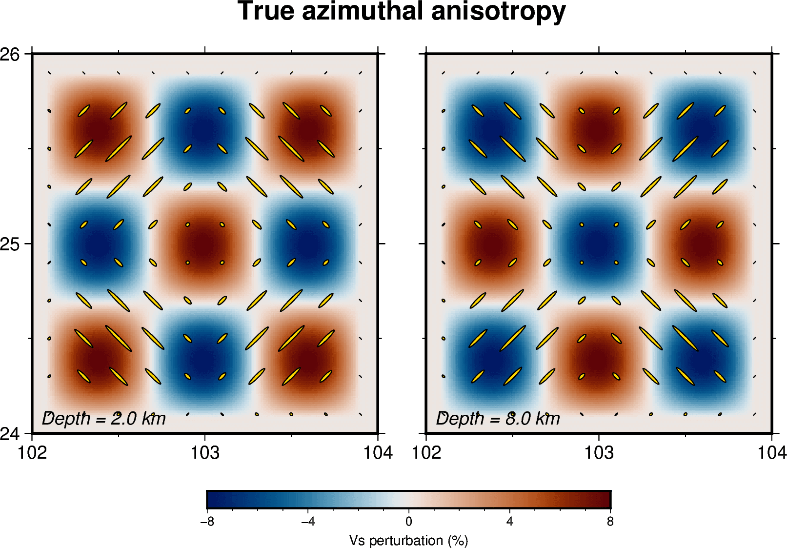
Target perturbations and azimuthal anisotropy at 2 and 8 km depth.
The vertical section at latitude shows the two checkerboard layers. The left panel displays the signed perturbation, while the right panel displays the non-negative anisotropy magnitude .
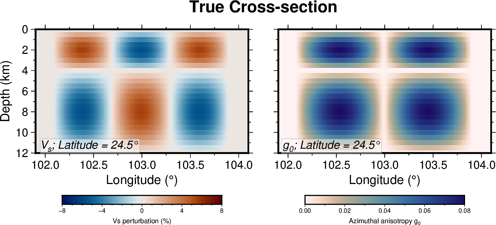
Target and sections at latitude .
3. Invert the synthetic observations
After the forward command finishes successfully, run:
mpirun -np 8 ../../bin/SURFATT_tomo -i input_params.ymlThe inversion reads the synthetic Rayleigh observations. It rebuilds the unperturbed starting model and attempts to recover the target structure from travel times alone.
For each inversion iteration, SurfATT:
- predicts Rayleigh-wave phase travel times from the current model;
- calculates residuals relative to the synthetic observations;
- computes adjoint sensitivity kernels for , , and ;
- applies the isotropic and anisotropic smoothing settings from
postproc; - uses LBFGS with line search to update the three model parameters; and
- records the misfit, current model, gradients, and predicted travel times.
The run stops when iteration reaches niter: 80, when the recent mean-misfit reduction falls below min_derr: 0.0015%, or when the line search can no longer find an acceptable update.
4. Check the inversion products
The main inversion outputs are:
| File | Description |
|---|---|
final_model.h5 | Recovered model containing vs, gc, gs, g0, and theta |
model_iter.h5 | Model and gradient history used to inspect convergence |
objective_function.txt | Total misfit, Rayleigh residual statistics, and step length for each iteration |
src_rec_file_forward_RL_PH_*.csv | Rayleigh predictions produced during inversion |
The original target_model.h5 remains in OUTPUT_FILES/ for the target-versus-recovery comparison.
Visualization
Open plot_model.ipynb after the inversion to reproduce these figures or inspect other depths and sections.
The recovered horizontal slices preserve the alternating pattern and the principal fast-axis orientations. Compared with the target, both the velocity boundaries and the anisotropy bars are smoother because of model regularization and finite path coverage.
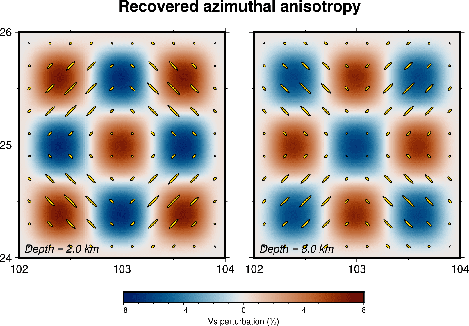
Recovered perturbations and azimuthal anisotropy at 2 and 8 km depth.
The recovered vertical sections retain the two depth layers in both and . The anisotropy magnitude is more strongly smoothed than the isotropic velocity perturbation, especially near anomaly boundaries.
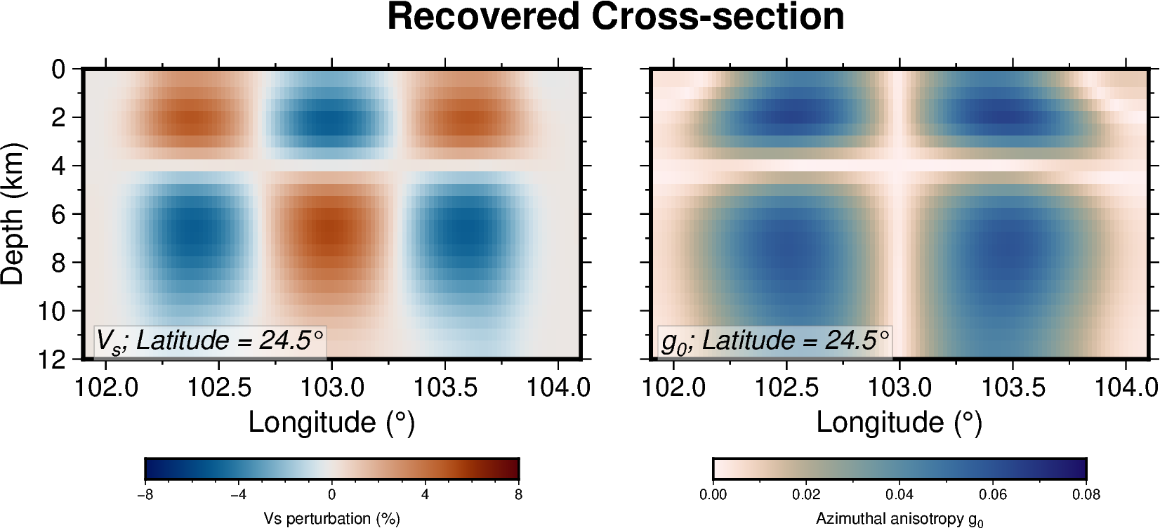
Recovered and sections at latitude .
For a quantitative assessment, compare target_model.h5 and final_model.h5 using consistent color and bar-length scales. Examine the recovered anomaly polarity, block location, perturbation amplitude, fast-axis direction, and leakage between and .