Example 02: Radial Anisotropy Checkerboard
This example reproduces SurfATTPP/examples/02_checkerboard_radial_ani. It uses both Rayleigh- and Love-wave phase velocities to test recovery of isotropic velocity structure and radial anisotropy.
Model parameterization
SurfATT represents radial anisotropy using two polarized S-wave velocities:
| Parameter | Unit | Definition and physical meaning |
|---|---|---|
| km/s | Velocity of an S wave polarized in the vertical plane. Rayleigh waves provide the primary constraint on this component. | |
| km/s | Velocity of an S wave polarized in the horizontal plane. Love waves provide the primary constraint on this component. | |
| km/s | Effective S-wave velocity describing the isotropic part of the model. | |
| dimensionless | Radial-anisotropy strength, defined from the squared velocity ratio. |
The effective velocity and radial-anisotropy strength are
The inverse conversion used by SurfATT is
The value of provides a direct interpretation of the anisotropy:
- : , so the S-wave model is isotropic.
- : , so horizontally polarized S waves are faster.
- : , so vertically polarized S waves are faster.
Internally, the radial-anisotropy inversion updates and
The HDF5 model files expose all four user-facing fields—vsv, vsh, vs, and zeta—so results can be plotted using either velocity components or the more intuitive parameterization.
What is included
| File | Description |
|---|---|
input_params.yml | Radially anisotropic inversion settings |
src_rec_file_ph.csv | Phase-velocity source–receiver table used for Rayleigh and Love waves |
src_rec_file_gr.csv | Group-velocity table, copied by the script but disabled in the default configuration |
run_this_example.sh | Script for the forward and inversion stages |
plot_model.ipynb | Notebook for plotting velocity and radial-anisotropy recovery |
Parameter setup
The default configuration uses:
- radial-anisotropy inversion (
model_para_type: 2) - Rayleigh- and Love-wave phase-velocity data
- model depth range of
0-8 km - longitude, latitude, and depth intervals of
0.02° / 0.02° / 0.5 km - up to
40LBFGS iterations
Setting model_para_type: 2 activates the – radial-anisotropy inversion and requires both Rayleigh and Love data.
Run the example
The example has two dependent stages. First, SURFATT_cb_fwd creates the target checkerboard and synthetic observations. Then, SURFATT_tomo starts from the unperturbed model and inverts those observations.
For a complete automatic run, execute the supplied script from the example directory:
bash run_this_example.shThe following sections unpack the script step by step.
1. Prepare the forward inputs
Create the output directory and copy the source-receiver geometry to the filenames configured in input_params.yml:
mkdir -p OUTPUT_FILES
cp src_rec_file_ph.csv OUTPUT_FILES/src_rec_file_forward_RL_PH.csv
cp src_rec_file_ph.csv OUTPUT_FILES/src_rec_file_forward_LV_PH.csv
The default configuration contains
wave_type: [True, True]   # Rayleigh and Love
vel_type:  [True, False]  # phase only
Therefore, only src_rec_file_forward_RL_PH.csv and src_rec_file_forward_LV_PH.csv are read in this example. The helper script also copies the two group-velocity tables so the example can be extended by changing vel_type to [True, True].
At this point the phase files provide the source-receiver geometry. Their travel-time and velocity columns will be replaced by synthetic values during the forward calculation.
2. Generate the target model and synthetic data
Run the radial-anisotropy checkerboard forward calculation:
mpirun -np 8 ../../bin/SURFATT_cb_fwd \
  -i input_params.yml \
  -n 2/3/2 \
  -s 2 \
  -r \
  -m 0.2 \
  -p 0.08/0.08
The command-line options define the synthetic model:
| Option | Meaning |
|---|---|
-i input_params.yml | Read the data paths, grid, initial model, and output settings |
-n 2/3/2 | Create a 2 × 3 × 2 checkerboard |
-r | Enable radial-anisotropy mode; it cannot be combined with -a |
-p 0.08/0.08 | Use 8% and 8% perturbations |
-m 0.2 | Leave a 0.2° horizontal margin between adjacent anomalies |
-s 2 | Set the upper anomaly size to 2 km |
The forward stage proceeds as follows:
-
SurfATT builds the 1-D starting model and extrudes it over the 3-D grid. The initial radial-anisotropy ratio is , so .
-
Alternating perturbations are applied in the parameterization:
-
Each checkerboard cell is converted from to for the wave-propagation calculation.
-
Rayleigh- and Love-wave phase travel times are calculated through the target model.
-
The synthetic travel times are written back to
src_rec_file_forward_RL_PH.csvandsrc_rec_file_forward_LV_PH.csv. These two files become the observations for the inversion.
The most important products of the forward stage are:
| File | Role in the workflow |
|---|---|
initial_model.h5 | Unperturbed isotropic starting model |
target_model.h5 | Known radial-anisotropy checkerboard used to generate the data |
src_rec_file_forward_RL_PH.csv | Synthetic Rayleigh-wave phase observations |
src_rec_file_forward_LV_PH.csv | Synthetic Love-wave phase observations |
Target checkerboard
The horizontal slices below show the prescribed and perturbations at depths of 1 and 5 km. Both parameters use the same alternating 2 × 3 lateral pattern, while the sign reverses between the shallow and deep checkerboard layers.
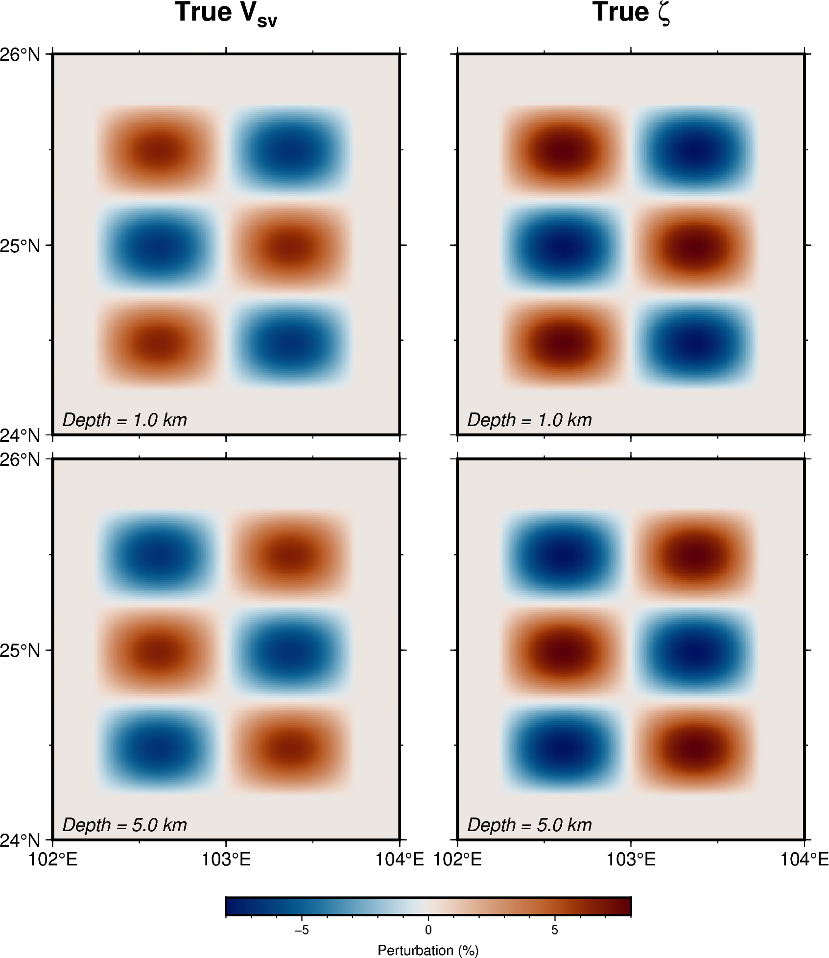
Target and perturbations at 1 and 5 km depth.
The vertical section at latitude shows the two depth layers directly. The upper anomalies occupy approximately 0–2 km, while the deeper checkerboard extends through the lower part of the 0–8 km model.
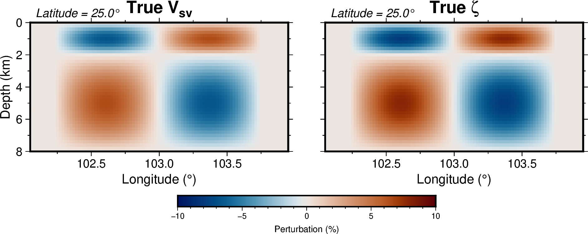
Target checkerboard section at latitude .
3. Invert the synthetic observations
After the forward command finishes successfully, run:
mpirun -np 8 ../../bin/SURFATT_tomo -i input_params.ymlThe inversion uses the same input_params.yml, but it does not receive the target model. It only reads the synthetic Rayleigh and Love observations and reconstructs the model from the unperturbed starting model.
For each inversion iteration, SurfATT:
- predicts Rayleigh- and Love-wave phase travel times from the current model;
- calculates residuals relative to the synthetic observations;
- computes adjoint sensitivity kernels for and ;
- smooths and conditions the gradients using the
postprocsettings; - uses LBFGS with line search to update and ; and
- records the misfit, current model, gradients, and predicted travel times.
The run stops when it reaches niter: 40, when the recent mean-misfit reduction falls below min_derr: 0.0015%, or when the line search can no longer find an acceptable update.
4. Check the inversion products
The main inversion outputs are:
| File | Description |
|---|---|
final_model.h5 | Recovered model containing vsv, vsh, vs, and zeta |
model_iter.h5 | Model and gradient history used to inspect convergence |
objective_function.txt | Total misfit, residual statistics, and step length for each iteration |
src_rec_file_forward_RL_PH_*.csv | Rayleigh predictions produced during inversion |
src_rec_file_forward_LV_PH_*.csv | Love predictions produced during inversion |
The original target_model.h5 remains in OUTPUT_FILES/, allowing a direct target-versus-recovery comparison. The inversion itself never reads this file.
Visualization
Open plot_model.ipynb after the inversion to reproduce these figures or inspect other depths and sections. For a quantitative assessment, compare target_model.h5 and final_model.h5 using the same color scale and examine:
The recovered horizontal slices retain the alternating polarity and locations of the target anomalies in both and . The recovered amplitudes are smoother and weaker than the target amplitudes, particularly for , because of the imposed gradient smoothing and the finite sensitivity of the Rayleigh–Love dataset.
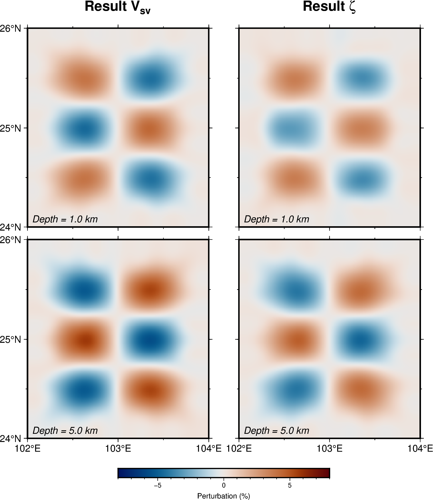
Recovered and perturbations at 1 and 5 km depth.
The vertical section confirms that the inversion resolves both checkerboard layers. Smoothing broadens the anomaly boundaries and reduces the recovered amplitude, but the depth-dependent sign changes remain visible.
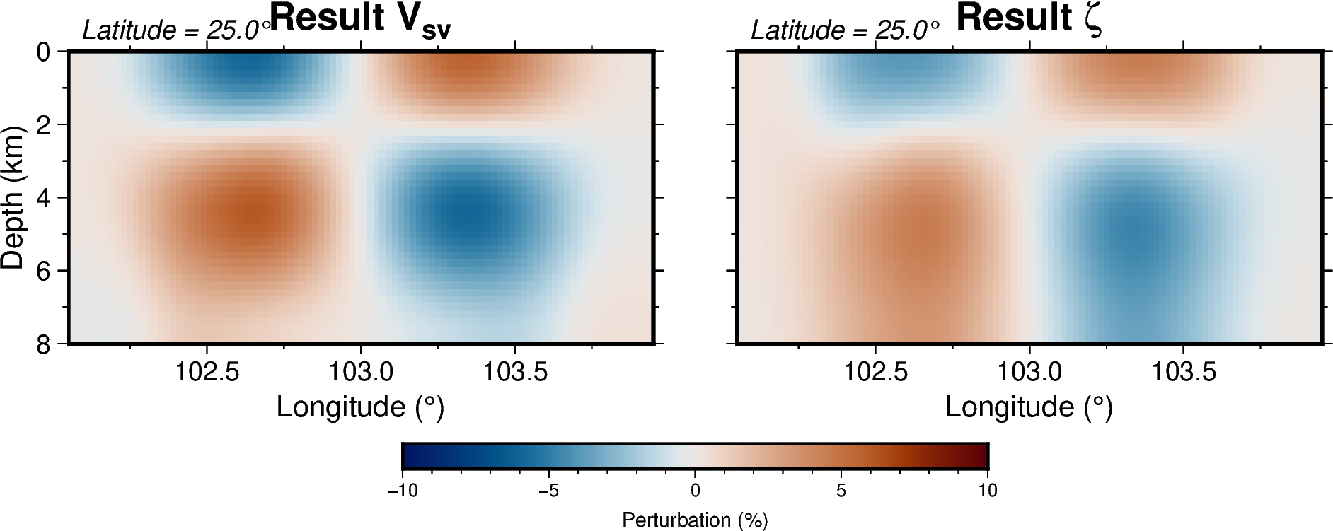
Recovered checkerboard section at latitude .